WaterLily

Introduction and Quickstart

WaterLily — Module

WaterLily.jl

Julia flow

Overview

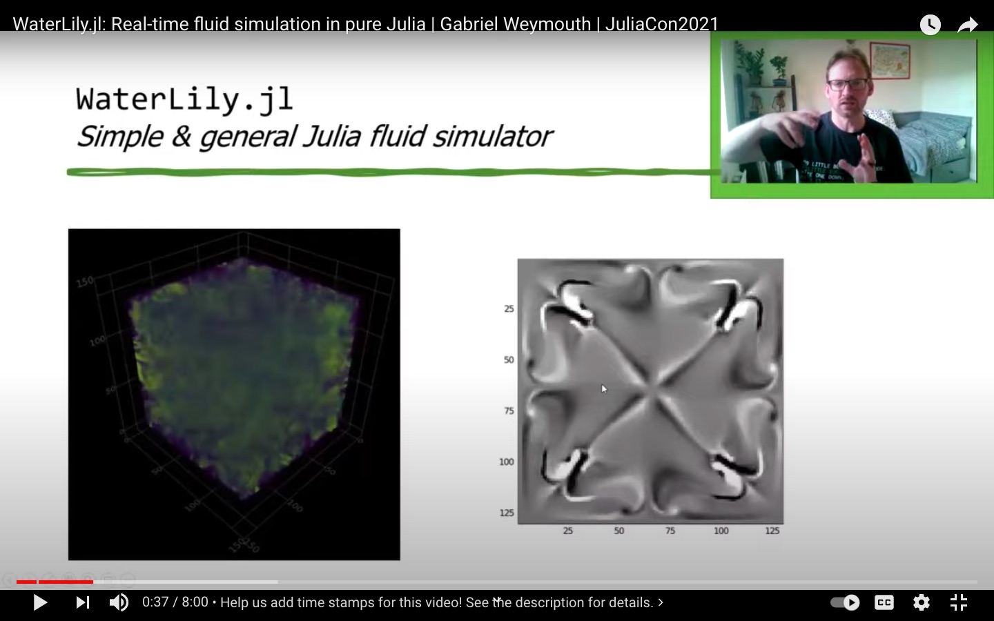
WaterLily.jl is a simple and fast fluid simulator written in pure Julia. This is an experimental project to take advantage of the active scientific community in Julia to accelerate and enhance fluid simulations. Watch the JuliaCon2021 talk here:

Method/capabilities

WaterLily.jl solves the unsteady incompressible 2D or 3D Navier-Stokes equations on a Cartesian grid. The pressure Poisson equation is solved with a geometric multigrid method. Solid boundaries are modelled using the Boundary Data Immersion Method. The solver can run on serial CPU, multi-threaded CPU, or GPU backends.

Examples

The user can set the boundary conditions, the initial velocity field, the fluid viscosity (which determines the Reynolds number), and immerse solid obstacles using a signed distance function. These examples and others are found in the examples.

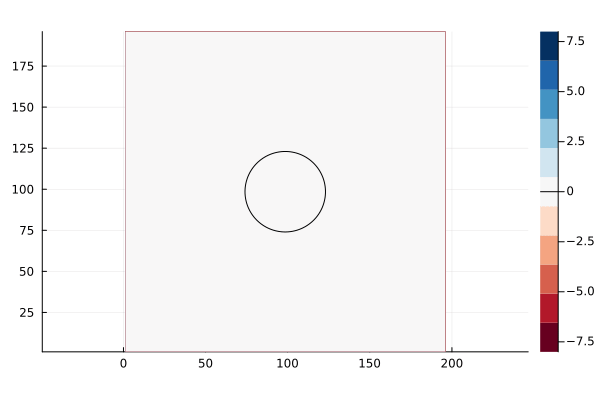
Flow over a circle

We define the size of the simulation domain as nxm cells. The circle has radius m/8 and is centered at (m/2,m/2). The flow boundary conditions are (U=1,0) and Reynolds number is Re=U*radius/ν where ν (Greek "nu" U+03BD, not Latin lowercase "v") is the kinematic viscosity of the fluid.

using WaterLily
function circle(n,m;Re=250,U=1)
    radius, center = m/8, m/2
    body = AutoBody((x,t)->√sum(abs2, x .- center) - radius)
    Simulation((n,m), (U,0), radius; ν=U*radius/Re, body)
end

The second to last line defines the circle geometry using a signed distance function. The AutoBody function uses automatic differentiation to infer the other geometric parameter automatically. Replace the circle's distance function with any other, and now you have the flow around something else... such as a donut or the Julia logo. Finally, the last line defines the Simulation by passing in parameters we've defined.

Now we can create a simulation (first line) and run it forward in time (third line)

circ = circle(3*2^6,2^7)
t_end = 10
sim_step!(circ,t_end)

Note we've set n,m to be multiples of powers of 2, which is important when using the (very fast) Multi-Grid solver. We can now access and plot whatever variables we like. For example, we could print the velocity at I::CartesianIndex using println(circ.flow.u[I]) or plot the whole pressure field using

using Plots
contour(circ.flow.p')

A set of flow metric functions have been implemented and the examples use these to make gifs such as the one above.

3D Taylor Green Vortex

The three-dimensional Taylor Green Vortex demonstrates many of the other available simulation options. First, you can simulate a nontrivial initial velocity field by passing in a vector function uλ(i,xyz) where i ∈ (1,2,3) indicates the velocity component uᵢ and xyz=[x,y,z] is the position vector.

function TGV(; pow=6, Re=1e5, T=Float64, mem=Array)
    # Define vortex size, velocity, viscosity
    L = 2^pow; U = 1; ν = U*L/Re
    # Taylor-Green-Vortex initial velocity field
    function uλ(i,xyz)
        x,y,z = @. (xyz-1.5)*π/L               # scaled coordinates
        i==1 && return -U*sin(x)*cos(y)*cos(z) # u_x
        i==2 && return  U*cos(x)*sin(y)*cos(z) # u_y
        return 0.                              # u_z
    end
    # Initialize simulation
    return Simulation((L, L, L), (0, 0, 0), L; U, uλ, ν, T, mem)
end

This example also demonstrates the floating point type (T=Float64) and array memory type (mem=Array) options. For example, to run on an NVIDIA GPU we only need to import the CUDA.jl library and initialize the Simulation memory on that device.

import CUDA
@assert CUDA.functional()
vortex = TGV(T=Float32,mem=CUDA.CuArray)
sim_step!(vortex,1)

For an AMD GPU, use import AMDGPU and mem=AMDGPU.ROCArray. Note that Julia 1.9 is required for AMD GPUs.

Moving bodies

Flapping line segment flow

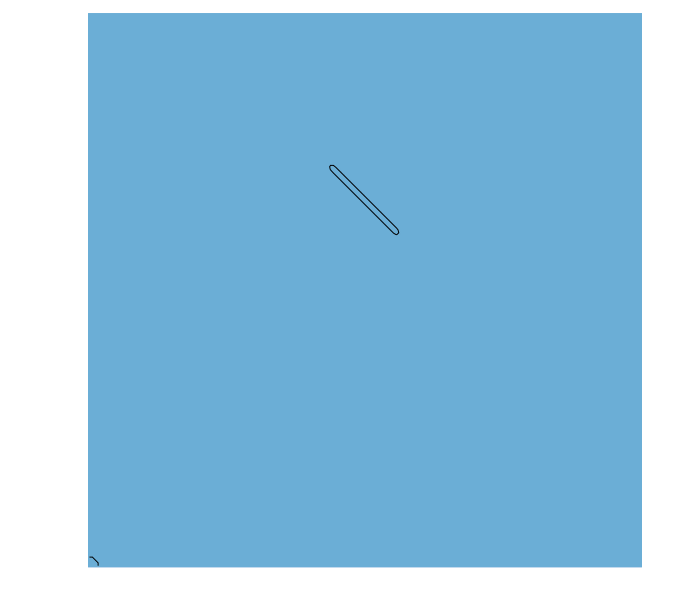
You can simulate moving bodies in WaterLily by passing a coordinate map to AutoBody in addition to the sdf.

using StaticArrays
function hover(L=2^5;Re=250,U=1,amp=π/4,ϵ=0.5,thk=2ϵ+√2)
    # Line segment SDF
    function sdf(x,t)
        y = x .- SA[0,clamp(x[2],-L/2,L/2)]
        √sum(abs2,y)-thk/2
    end
    # Oscillating motion and rotation
    function map(x,t)
        α = amp*cos(t*U/L); R = SA[cos(α) sin(α); -sin(α) cos(α)]
        R * (x - SA[3L-L*sin(t*U/L),4L])
    end
    Simulation((6L,6L),(0,0),L;U,ν=U*L/Re,body=AutoBody(sdf,map),ϵ)
end

In this example, the sdf function defines a line segment from -L/2 ≤ x[2] ≤ L/2 with a thickness thk. To make the line segment move, we define a coordinate transformation function map(x,t). In this example, the coordinate x is shifted by (3L,4L) at time t=0, which moves the center of the segment to this point. However, the horizontal shift varies harmonically in time, sweeping the segment left and right during the simulation. The example also rotates the segment using the rotation matrix R = [cos(α) sin(α); -sin(α) cos(α)] where the angle α is also varied harmonically. The combined result is a thin flapping line, similar to a cross-section of a hovering insect wing.

One important thing to note here is the use of StaticArrays to define the sdf and map. This speeds up the simulation since it eliminates allocations at every grid cell and time step.

Circle inside an oscillating flow

Oscillating flow

This example demonstrates a 2D oscillating periodic flow over a circle.

function circle(n,m;Re=250,U=1)
    # define a circle at the domain center
    radius = m/8
    body = AutoBody((x,t)->√sum(abs2, x .- (n/2,m/2)) - radius)

    # define time-varying body force `g` and periodic direction `perdir`
    accelScale, timeScale = U^2/2radius, radius/U
    g(i,t) = i==1 ? -2accelScale*sin(t/timeScale) : 0 
    Simulation((n,m), (U,0), radius; ν=U*radius/Re, body, g, perdir=(1,))
end

The g argument accepts a function with direction (i) and time (t) arguments. This allows you to create a spatially uniform body force with variations over time. In this example, the function adds a sinusoidal force in the "x" direction i=1, and nothing to the other directions.

The perdir argument is a tuple that specifies the directions to which periodic boundary conditions should be applied. Any number of directions may be defined as periodic, but in this example only the i=1 direction is used allowing the flow to accelerate freely in this direction.

Accelerating reference frame

accelerating cylinder

WaterLily gives the posibility to set up a Simulation using time-varying boundary conditions for the velocity field. This can be used to simulate a flow in an accelerating reference frame. The following example demonstrates how to set up a Simulation with a time-varying velocity field.

using WaterLily
# define time-varying velocity boundary conditions
Ut(i,t::T;a0=0.5) where T = i==1 ? convert(T, a0*t) : zero(T)
# pass that to the function that creates the simulation
sim = Simulation((256,256), Ut, 32)

The Ut function is used to define the time-varying velocity field. In this example, the velocity in the "x" direction is set to a0*t where a0 is the acceleration of the reference frame. The Simulation function is then called with the Ut function as the second argument. The simulation will then run with the time-varying velocity field.

Periodic and convective boundary conditions

periodic cylinder

In addition to the standard free-slip (or reflective) boundary conditions, WaterLily also supports periodic boundary conditions. The following example demonstrates how to set up a Simulation with periodic boundary conditions in the "y" direction.

using WaterLily,StaticArrays

# sdf an map for a moving circle in y-direction
function sdf(x,t)
    norm2(SA[x[1]-192,mod(x[2]-384,384)-192])-32
end
function map(x,t)
    x.-SA[0.,t/2]
end

# make a body
body = AutoBody(sdf, map)

# y-periodic boundary conditions
Simulation((512,384), (1,0), 32; body, perdir=(2,))

Additionally, the flag exitBC=true can be passed to the Simulation function to enable convective boundary conditions. This will apply a 1D convective exit in the x direction (there is not way to change this at the moment). The exitBC flag is set to false by default. In this case, the boundary condition is set to the corresponding value of the u_BC vector you specified when constructing the Simulation.

using WaterLily

# make a body
body = AutoBody(sdf, map)

# y-periodic boundary conditions
Simulation((512,384), u_BC=(1,0), L=32; body, exitBC=true)

Writing to a VTK file

The following example demonstrates how to write simulation data to a .pvd file using the WriteVTK package and the WaterLily vtkwriter function. The simplest writer can be instantiated with

using WaterLily,WriteVTK

# make a sim
sim = make_sim(...)

# make a writer
writer = vtkwriter("simple_writer")

# write the data
write!(writer,sim)

# don't forget to close the file
close(writer)

This would write the velocity and pressure fields to a file named simmple_writer.pvd. The vtkwriter function can also take a dictionary of custom attributes to write to the file. For example, to write the body (sdf) and λ₂ fields to the file, you could use the following code:

using WaterLily,WriteVTK

# make a writer with some attributes, need to output to CPU array to save file (|> Array)
velocity(a::Simulation) = a.flow.u |> Array;
pressure(a::Simulation) = a.flow.p |> Array;
_body(a::Simulation) = (measure_sdf!(a.flow.σ, a.body, WaterLily.time(a)); 
                                     a.flow.σ |> Array;)
lamda(a::Simulation) = (@inside a.flow.σ[I] = WaterLily.λ₂(I, a.flow.u);
                        a.flow.σ |> Array;)
                        
# this maps field names to values in the file
custom_attrib = Dict(
    "Velocity" => velocity,
    "Pressure" => pressure,
    "Body" => _body,
    "Lambda" => lamda
)

# make the writer
writer = vtkWriter("advanced_writer"; attrib=custom_attrib)
...
close(writer)

The functions that are passed to the attrib (custom attributes) must follow the same structure as what is shown in this example, that is, given a Simulation, return a N-dimensional (scalar or vector) field. The vtkwriter function will automatically write the data to a .pvd file, which can be read by Paraview. The prototype for the vtkwriter function is:

# prototype vtk writer function
custom_vtk_function(a::Simulation) = ... |> Array

the ... should be replaced with the code that generates the field you want to write to the file. The piping to a (CPU) Array is necessary to ensure that the data is written to the CPU before being written to the file for GPU simulations.

Restarting from a VTK file

This capability is very usefull to restart a simulation from a previous state. The ReadVTK package is used to read simulation data from a .pvd file. This .pvd must have been writen with the vtkwriter function and must contain at least the velocity and pressure fields. The following example demonstrates how to restart a simulation from a .pvd file using the ReadVTK package and the WaterLily vtkreader function

using WaterLily,ReadVTK
sim = make_sim(...)
# restart the simulation
writer = restart_sim!(sim; fname="file_restart.pvd")

# this acctually append the data to the file used to restart
write!(writer, sim)

# don't forget to close the file
close(writer)

Internally, this function reads the last file in the .pvd file and use that to set the velocity and pressure fields in the simulation. The sim_time is also set to the last value saved in the .pvd file. The function also returns a vtkwriter that will append the new data to the file used to restart the simulation. Note the sim that will be filled must be identical to the one saved to the file for this restart to work, that is, the same size, same body, etc.

Multi-threading and GPU backends

WaterLily uses KernelAbstractions.jl to multi-thread on CPU and run on GPU backends. The implementation method and speed-up are documented in our ParCFD abstract. In summary, a single macro WaterLily.@loop is used for nearly every loop in the code base, and this uses KernelAbstractactions to generate optimized code for each back-end. The speed-up is more pronounce for large simulations, and we've benchmarked up to 23x-speed up on a Intel Core i7-10750H x6 processor, and 182x speed-up NVIDIA GeForce GTX 1650 Ti GPU card.

Note that multi-threading requires starting Julia with the --threads argument, see the multi-threading section of the manual. If you are running Julia with multiple threads, KernelAbstractions will detect this and multi-thread the loops automatically. As in the Taylor-Green-Vortex examples above, running on a GPU requires initializing the Simulation memory on the GPU, and care needs to be taken to move the data back to the CPU for visualization. See jelly fish for another non-trivial example.

Finally, KernelAbstractions does incur some CPU allocations for every loop, but other than this sim_step! is completely non-allocating. This is one reason why the speed-up improves as the size of the simulation increases.

Development goals

Immerse obstacles defined by 3D meshes using GeometryBasics.
Multi-CPU/GPU simulations.
Add free-surface physics with Volume-of-Fluid or Level-Set.
Add external potential-flow domain boundary conditions.

If you have other suggestions or want to help, please raise an issue on github.

WaterLily

Introduction and Quickstart

Types Methods and Functions